
As part of a typical university algorithms exercise, I ran a small comparative analysis of the most popular sorting algorithms. The idea was to study complexity and see how different approaches to the same problem can produce very different execution times.
This is a simple academic analysis, but I wanted to document it in case it helps other computer science students in the future.
I started with a small Java script to generate random five-digit numbers and store them in a text file, so I could benchmark all algorithms against exactly the same dataset. The script is available in this repository:
# File path
> algorithms/java/RandomNumbers.java

# Run Java script
$ javac RandomNumbers.java && java RandomNumbers
That produces numbers/numbers.txt with n random numbers configured in the script. In my experiments I generated up to 1,000,000,000 values (about 5 GB), so I did not include that dataset in the repository.
Evaluated algorithms
I implemented the following algorithms:
- Bubble Sort:
O(n^2) - Counting Sort:
O(n+k) - Heap Sort:
O(n log n) - Insertion Sort:
O(n^2) - Merge Sort:
O(n log n) - Quicksort:
O(n log n) - Selection Sort:
O(n^2)
I used C for implementations, under algorithms/c/sortAlgorithms.
Benchmark automation
Since this required many runs, I automated execution with two scripts:
# Base benchmark script
> algorithms/c/benchmark.c

# Run one benchmark
$ gcc benchmark.c -o benchmark.out && ./benchmark.out arg1 arg2

# Multi-run script
> algorithms/c/runTest.c

# Run all tests
$ gcc runTest.c -o runTest.out && ./runTest.out
I ran this in a small controlled environment to minimize interference from other processes.
I created two Digital Ocean droplets:

The second machine had double resources, so better performance seemed expected.
I also provisioned Java and C using this script: ServerConfig/provision.sh
sudo apt-get update -y
sudo apt-get upgrade -y
sudo apt-get install -y build-essential gcc python-dev python-pip python-setuptools
sudo apt-get install -y git
sudo apt-get install default-jre -y
sudo apt-get install default-jdk -y
sudo apt-get install openjdk-7-jre -y
sudo apt-get install openjdk-7-jdk -y
Results
Both machines used the same random dataset, with growing input sizes. Full results are in results/analysis.ods.
I also used this background execution trick:
$ gcc runTest.c -o runTest.out && ./runTest.out
# Ctrl + z
disown -h %1
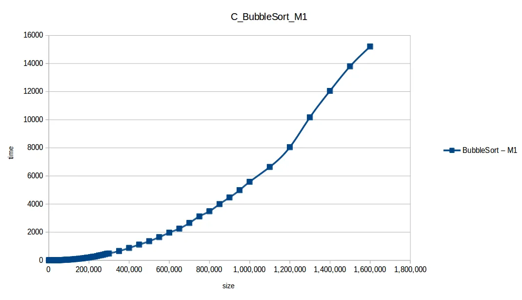
bg 1After 3-4 days, the O(n^2) algorithms had only reached 1,600,000 elements, so I stopped there and analyzed.
M1 = Machine 1 (1 core, 1GB RAM)
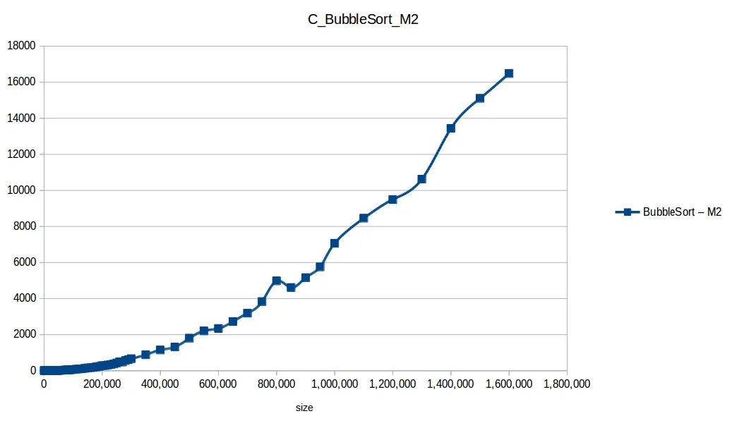
M2 = Machine 2 (2 cores, 2GB RAM)
Bubble Sort: O(n^2)
Counting Sort: O(n+k)
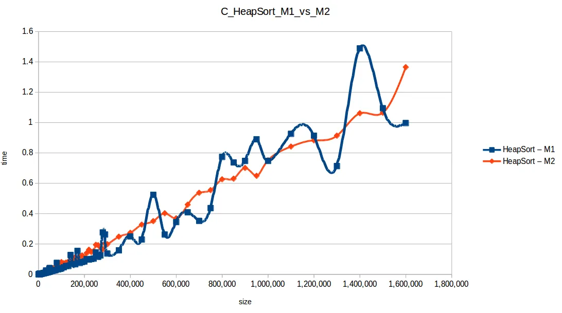
Heap Sort: O(n log n)
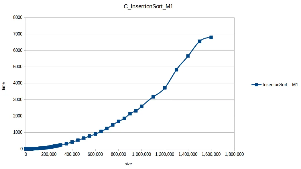
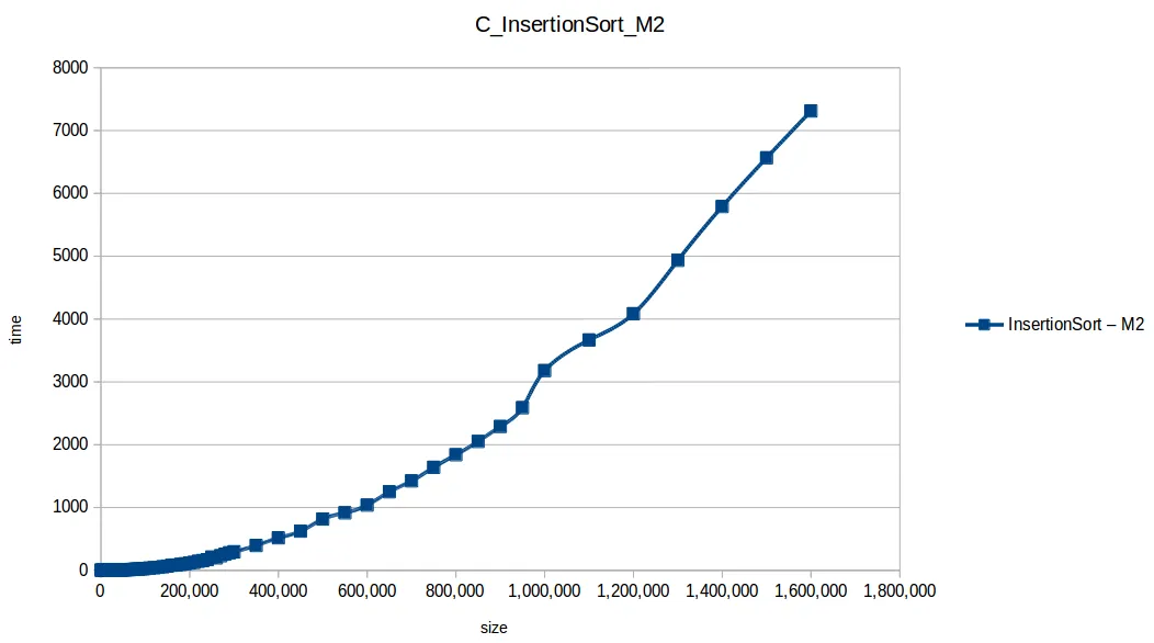
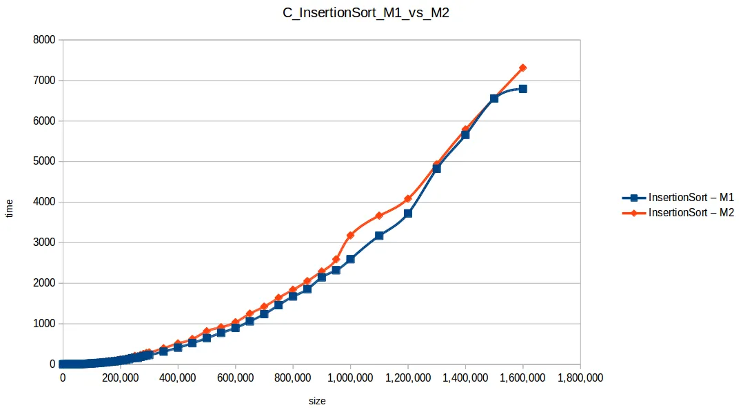
Insertion Sort: O(n^2)
Merge Sort: O(n log n)
Quicksort: O(n log n)
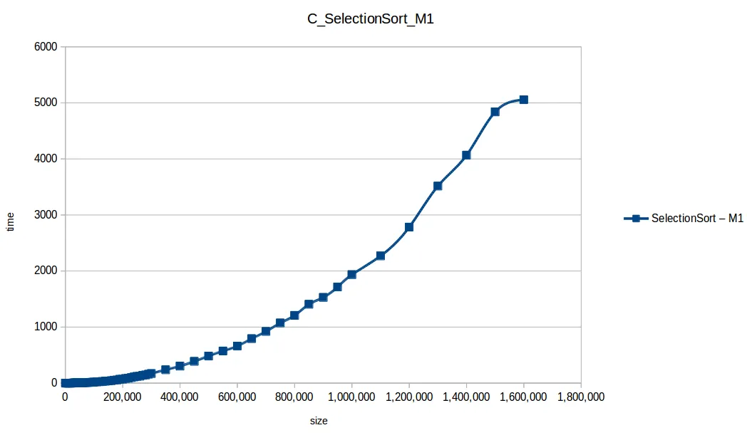
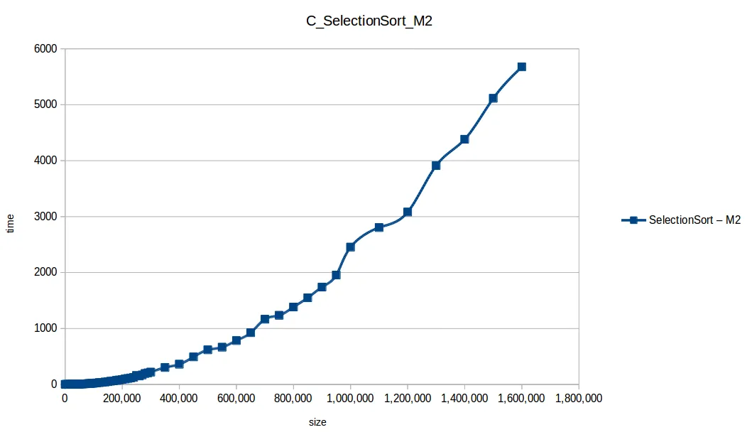
Selection Sort: O(n^2)
Full comparison chart
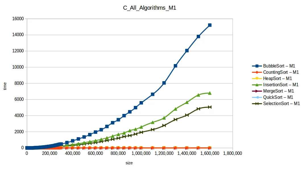
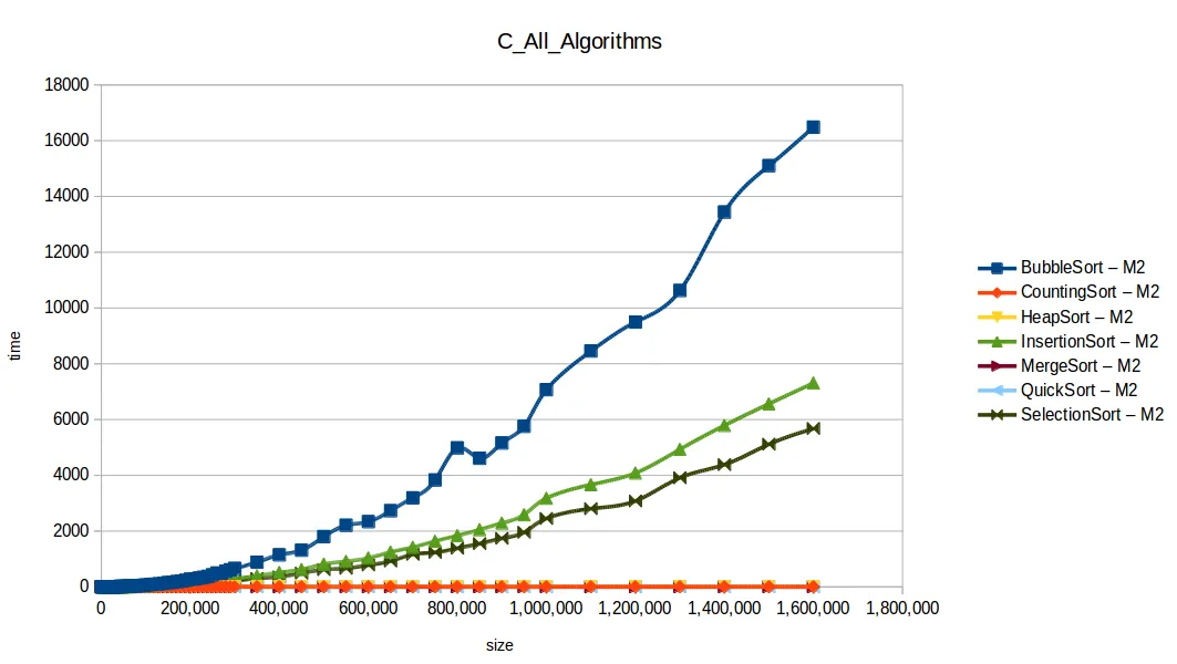
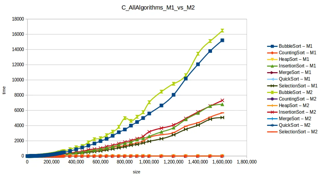
As expected, Bubble Sort is the clear loser. The fast group (quickSort, mergeSort, heapSort, countingSort) overlaps because of chart scale.
Last 7 response-time points
Machine 1
| Size | BubbleSort | CountingSort | HeapSort | InsertionSort | MergeSort | QuickSort | SelectionSort |
|---|---|---|---|---|---|---|---|
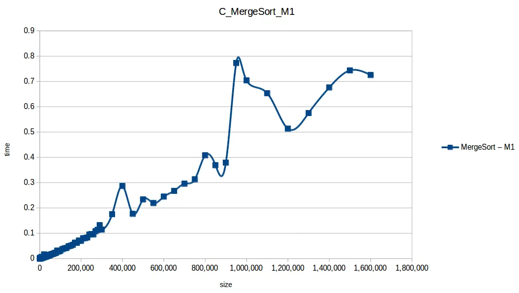
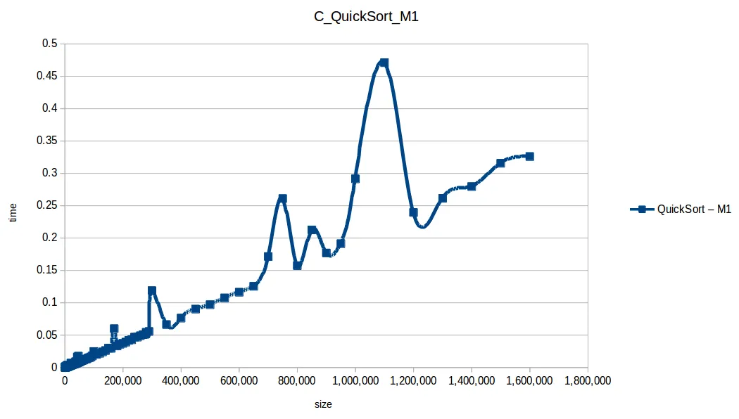
| 1,000,000 | 5584.254499 | 0.016609 | 0.747395 | 2592.498977 | 0.704281 | 0.291499 | 1935.487457 |
| 1,100,000 | 6637.222252 | 0.019187 | 0.925764 | 3171.445715 | 0.653455 | 0.471039 | 2269.966268 |
| 1,200,000 | 8045.953682 | 0.023652 | 0.913537 | 3722.638885 | 0.513099 | 0.239454 | 2783.279525 |
| 1,300,000 | 10169.383378 | 0.045208 | 0.713308 | 4824.250285 | 0.575149 | 0.261289 | 3514.914589 |
| 1,400,000 | 12053.658798 | 0.034613 | 1.489084 | 5658.739951 | 0.676112 | 0.279478 | 4066.729922 |
| 1,500,000 | 13798.854123 | 0.027525 | 1.094257 | 6555.365499 | 0.743651 | 0.315602 | 4839.340426 |
| 1,600,000 | 15205.680544 | 0.028478 | 0.996648 | 6794.512119 | 0.725347 | 0.325990 | 5056.213092 |
Machine 2
| Size | BubbleSort | CountingSort | HeapSort | InsertionSort | MergeSort | QuickSort | SelectionSort |
|---|---|---|---|---|---|---|---|
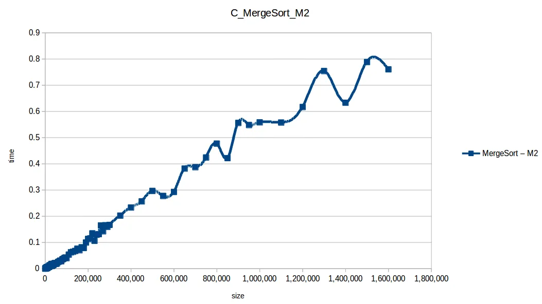
| 1,000,000 | 7069.317038 | 0.032415 | 0.752168 | 3178.694237 | 0.558200 | 0.315689 | 2454.531144 |
| 1,100,000 | 8458.150387 | 0.024157 | 0.842038 | 3666.359787 | 0.557481 | 0.284579 | 2804.449695 |
| 1,200,000 | 9495.898708 | 0.026530 | 0.882819 | 4084.581924 | 0.616636 | 0.358502 | 3081.748250 |
| 1,300,000 | 10626.023771 | 0.027309 | 0.913814 | 4933.201883 | 0.753890 | 0.401456 | 3912.714921 |
| 1,400,000 | 13439.250082 | 0.030009 | 1.061221 | 5790.797804 | 0.633180 | 0.442449 | 4066.729922 |
| 1,500,000 | 15102.736592 | 0.031826 | 1.064744 | 6565.630358 | 0.788551 | 0.400238 | 5114.565289 |
| 1,600,000 | 16483.694808 | 0.039298 | 1.365129 | 7311.347004 | 0.760618 | 0.449284 | 5676.768371 |
Fast algorithms only
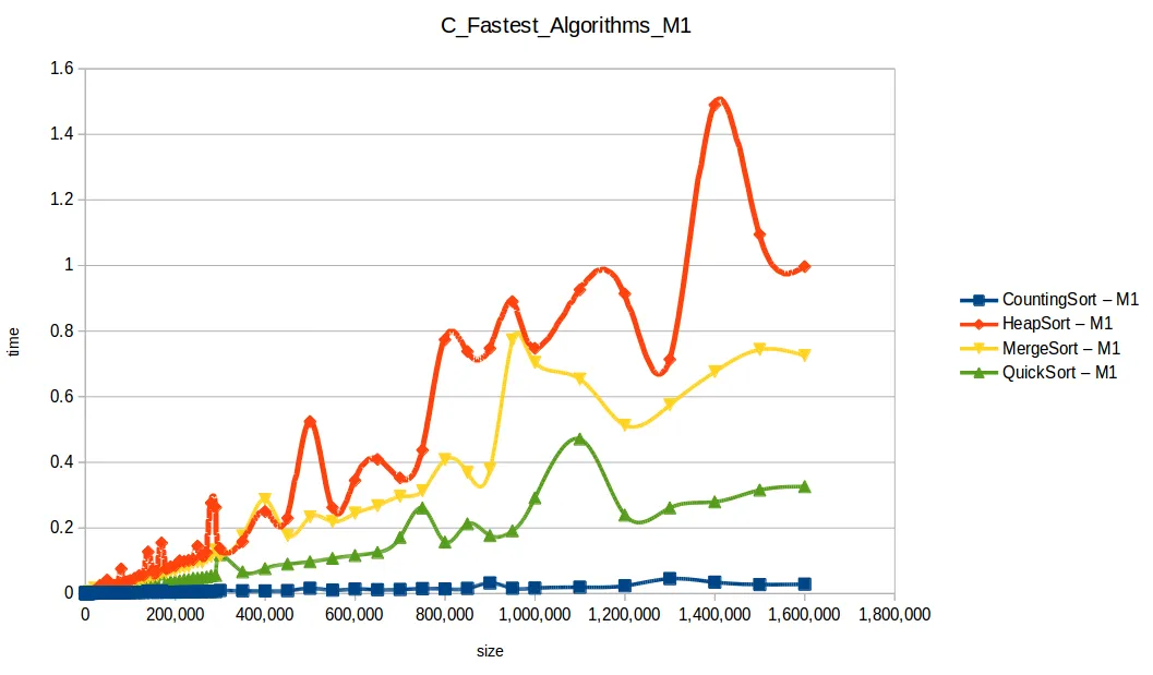
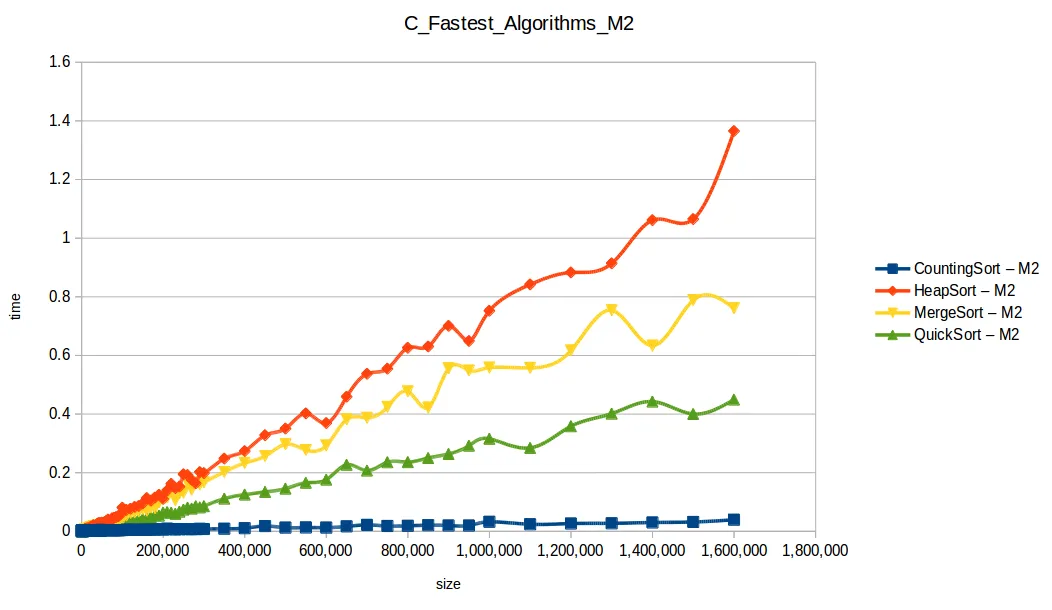
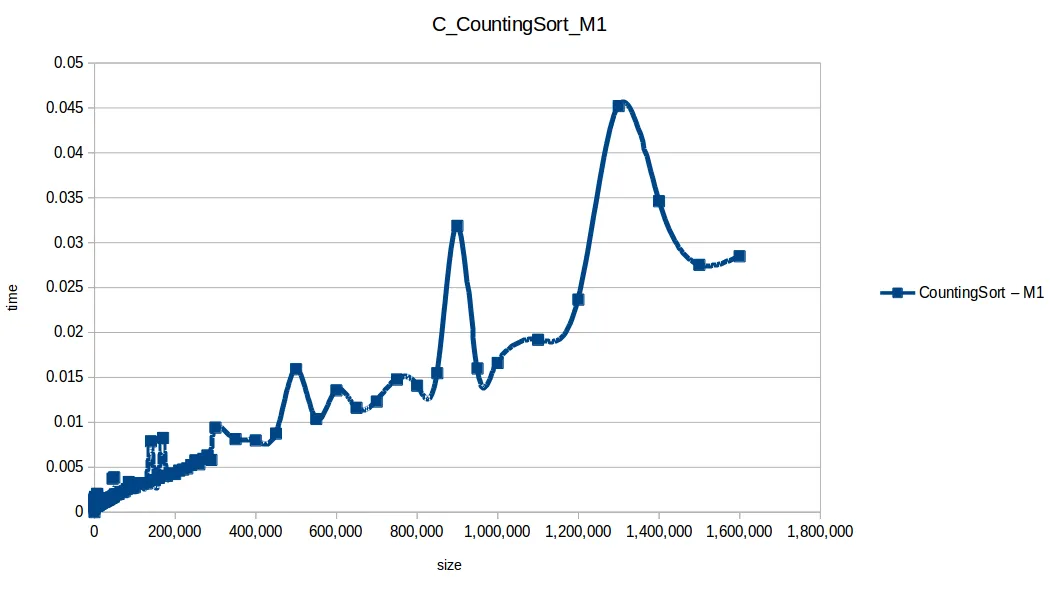
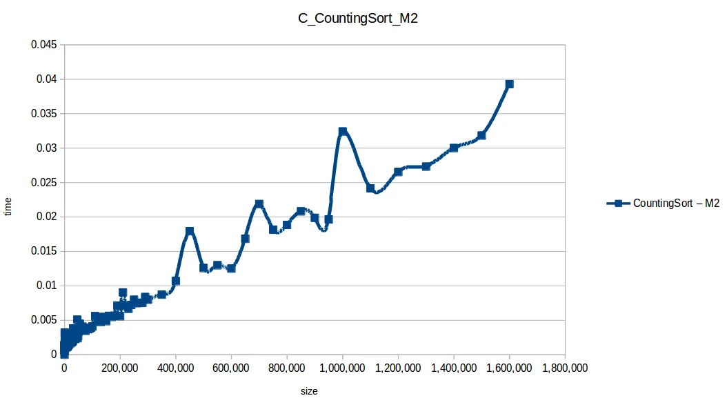
Counting Sort wins in this setup (O(n+k)), but it has practical limits:
- It only works on integer ranges.
- Memory usage can explode when
max - minis large.
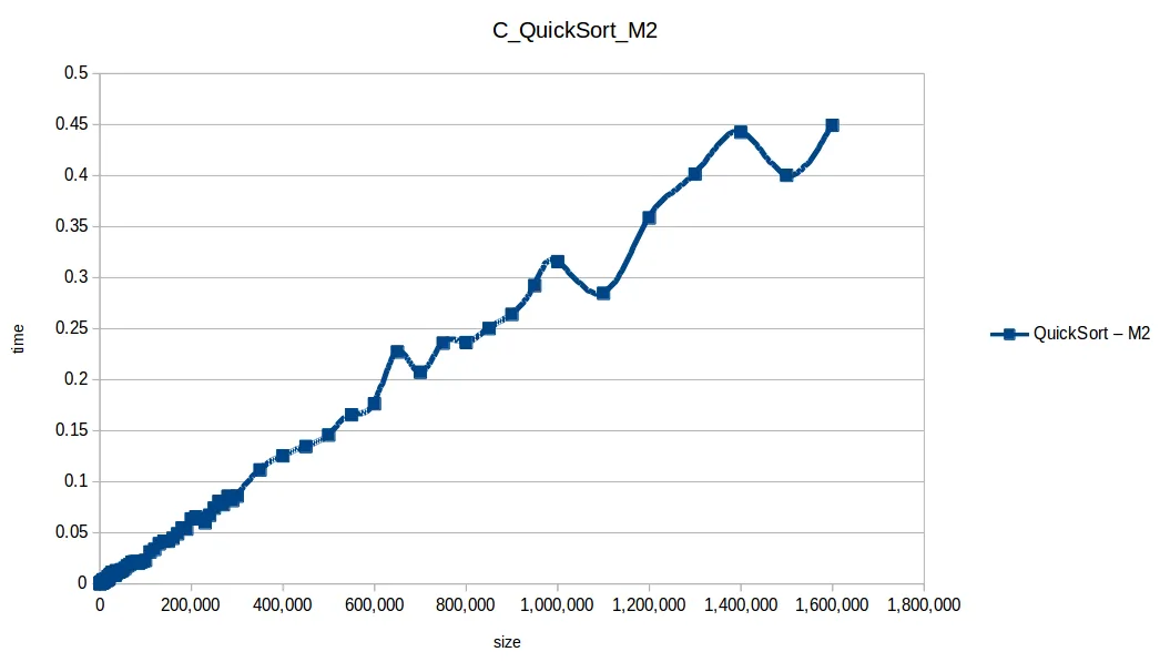
Quicksort was second and is broadly useful, but it can degrade to O(n^2) in bad pivot/distribution cases.
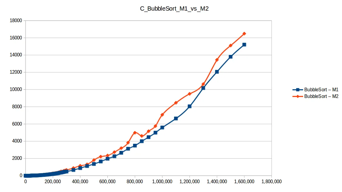
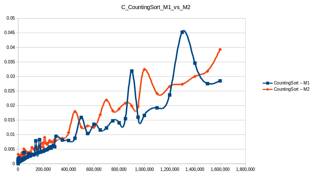
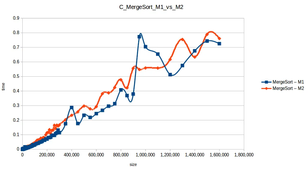
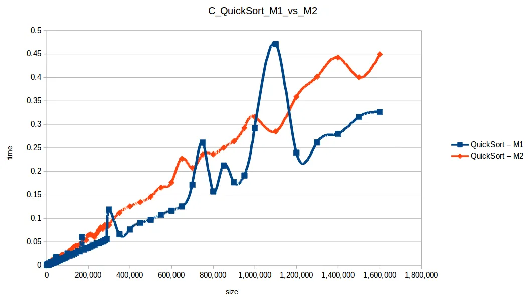
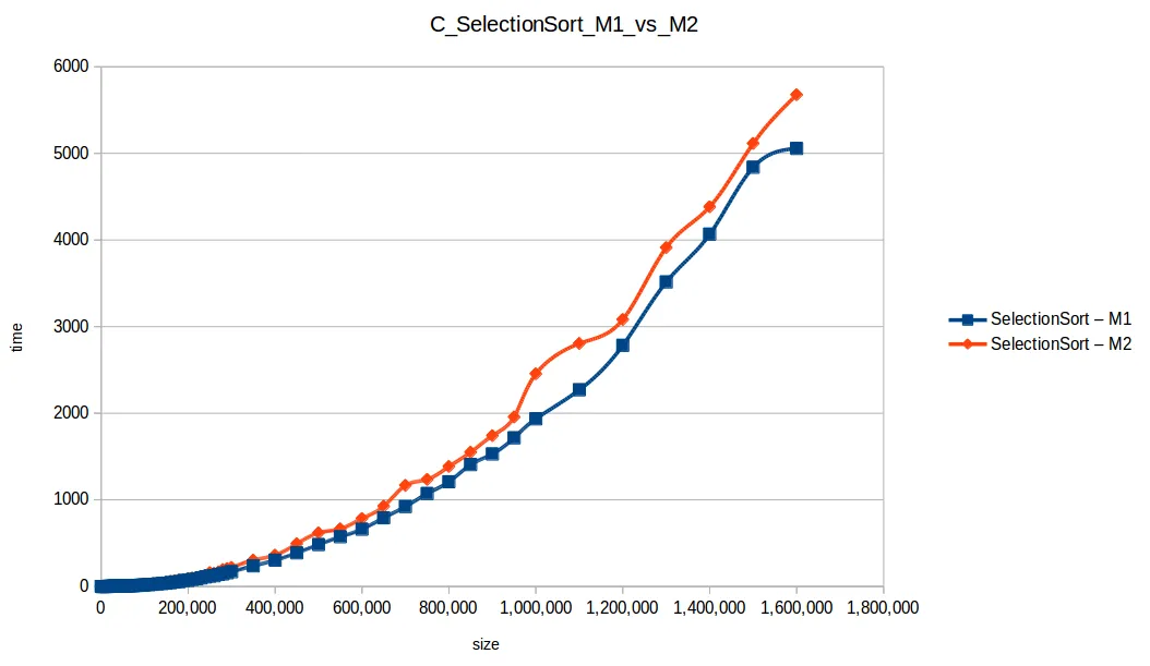
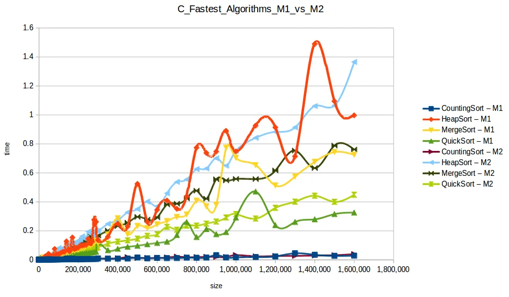
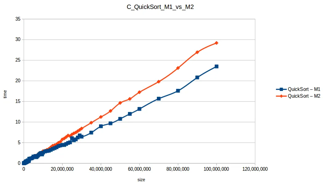
Machine 1 vs Machine 2
Why was M1 sometimes faster than M2 despite fewer resources?
Because these algorithm implementations were not parallelized. Even with two cores, M2 was effectively using one core for each single-threaded run.
Per-core frequency mattered:
- M1:
2399.998 MHz - M2:
1799.998 MHz
System architecture screenshots
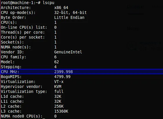
lscpu: 1 core at 2399.998 MHz — higher clock speed compensated for the smaller resource pool.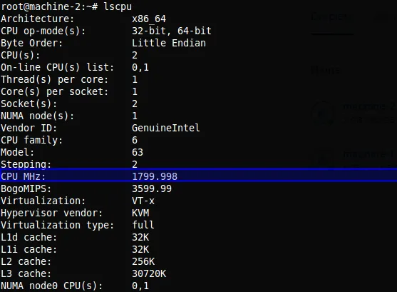
lscpu: 2 cores at 1799.998 MHz — more cores and RAM but lower per-core frequency.Frequency units:
- 1 Hz = one cycle/second
- 1 KHz = 1024 Hz
- 1 MHz = 1024 KHz
- 1 GHz = 1024 MHz
- 1 THz = 1024 GHz
Command used:
$ lscpuExtended memory-capacity phase
To better use machine resources, I ran only the efficient algorithms at larger scales:
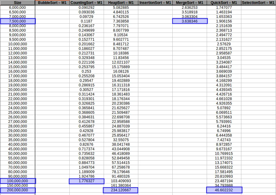
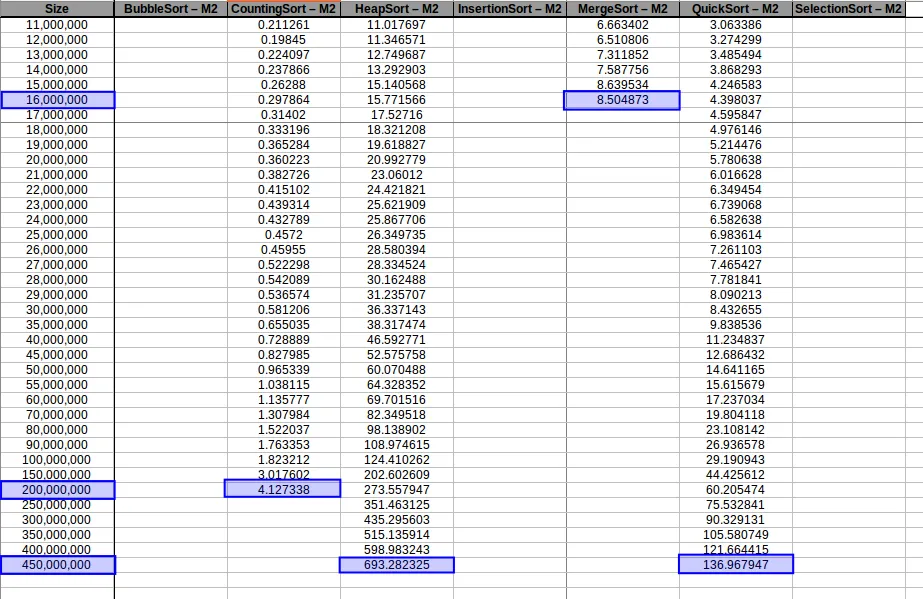
This is where M2’s extra RAM clearly helped.
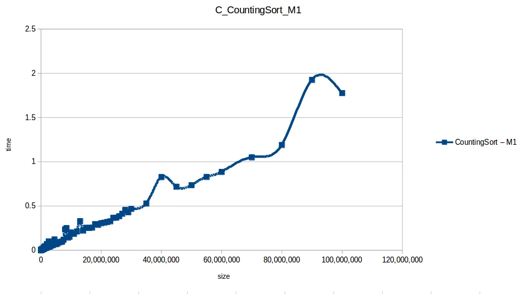
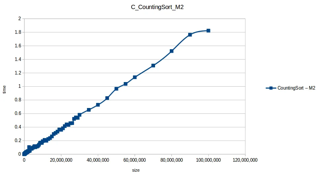
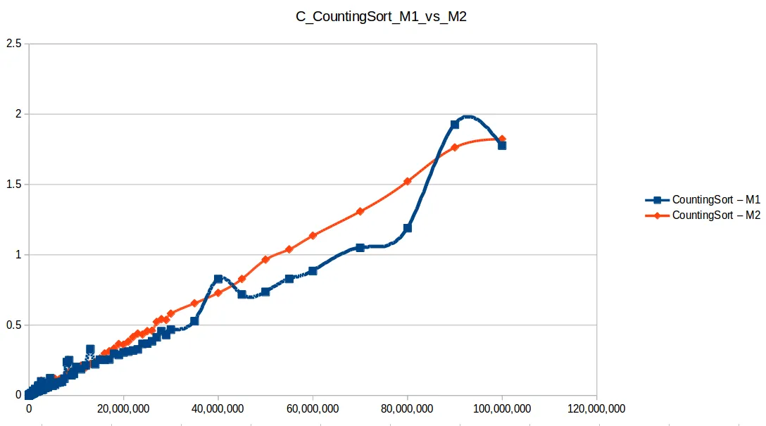
Counting Sort at max scale
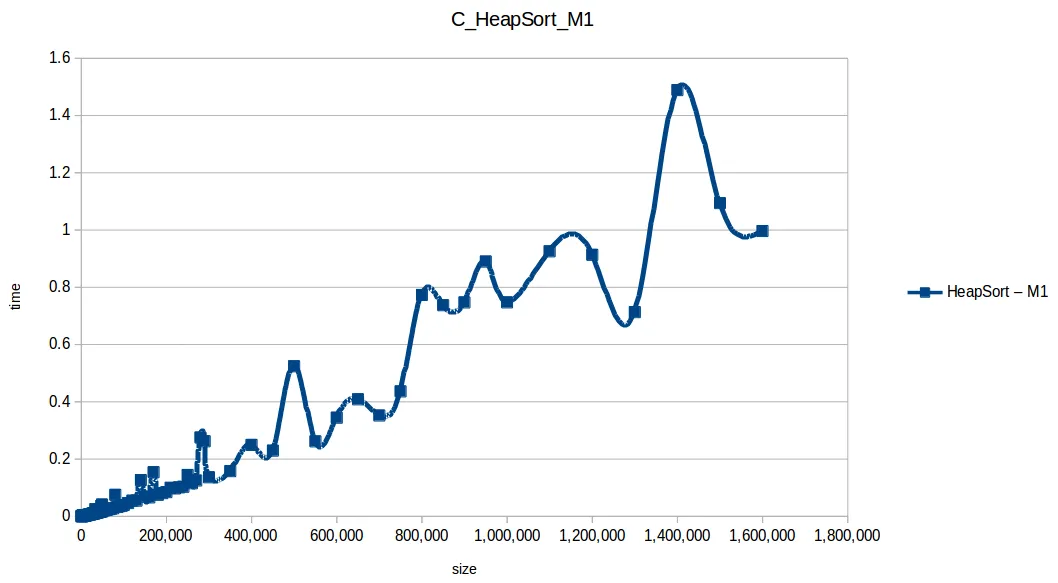
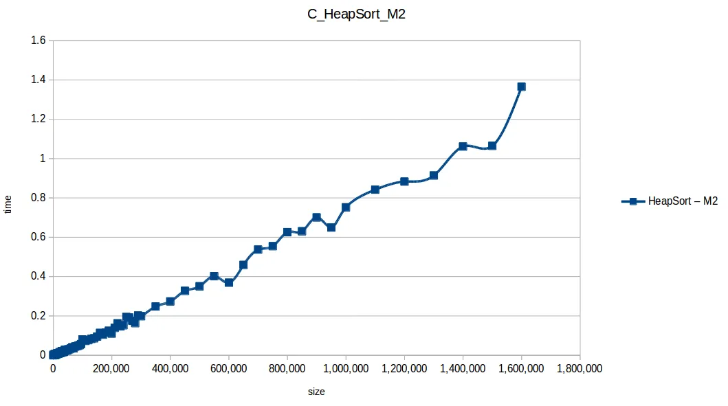
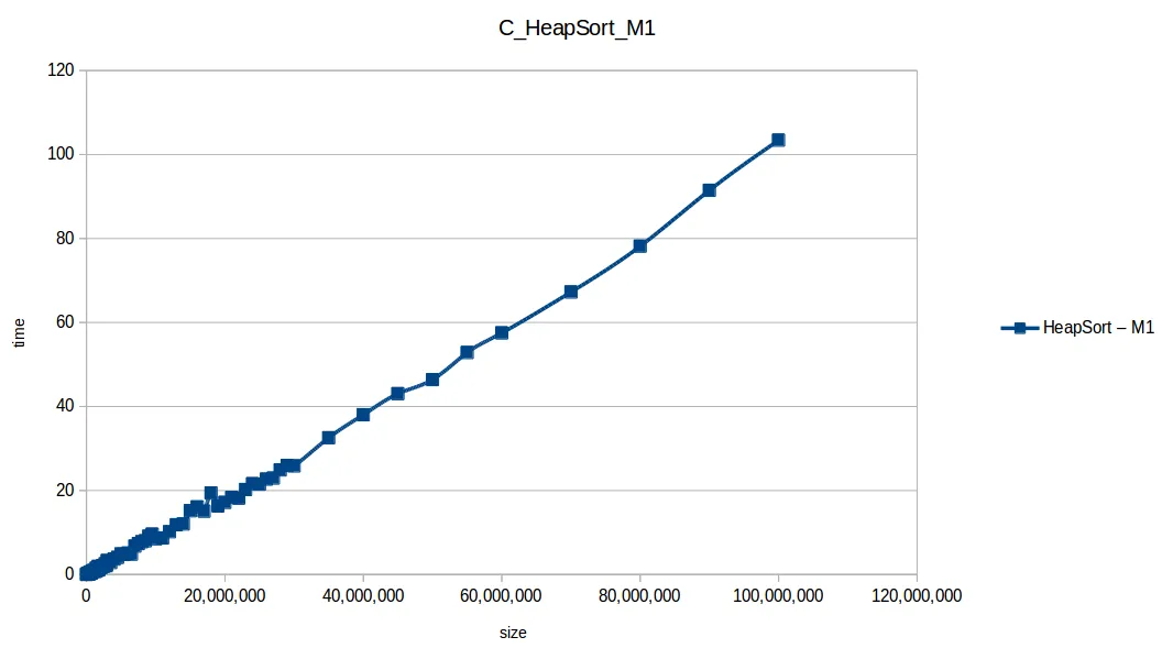
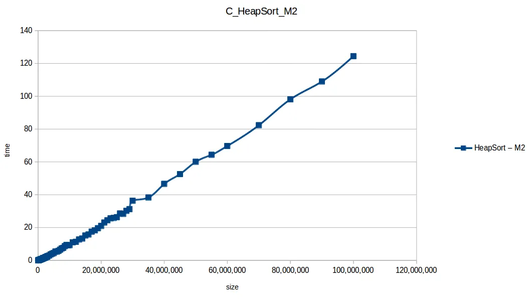
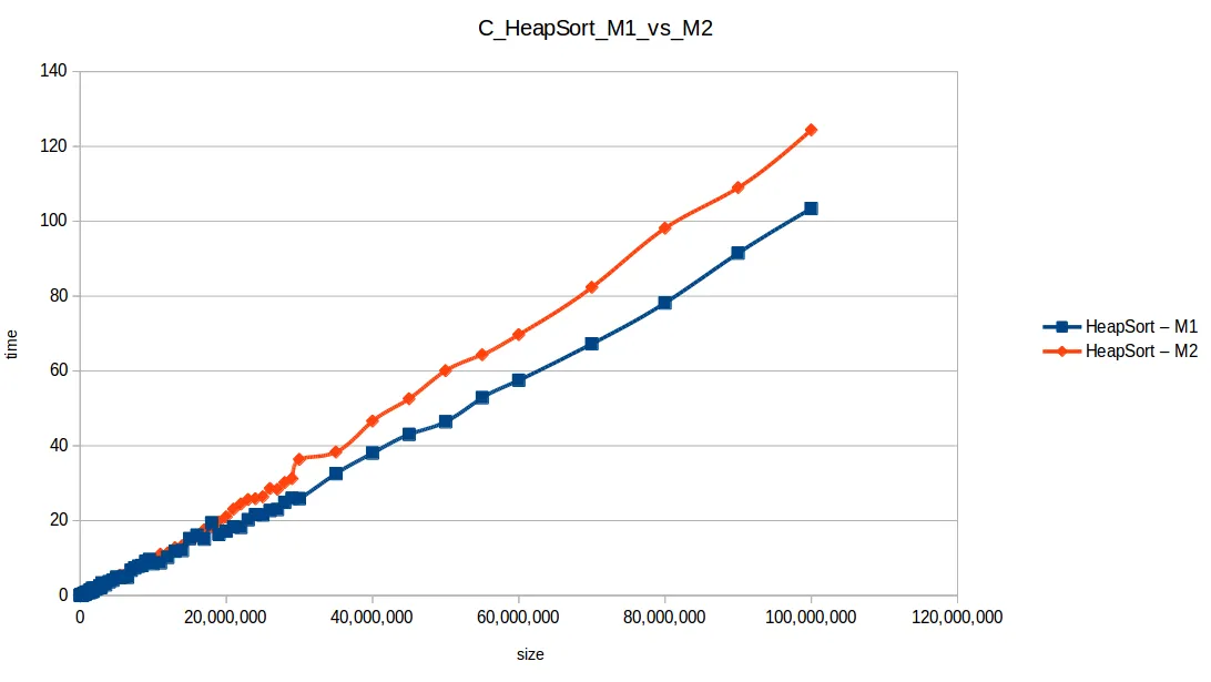
Heap Sort at max scale
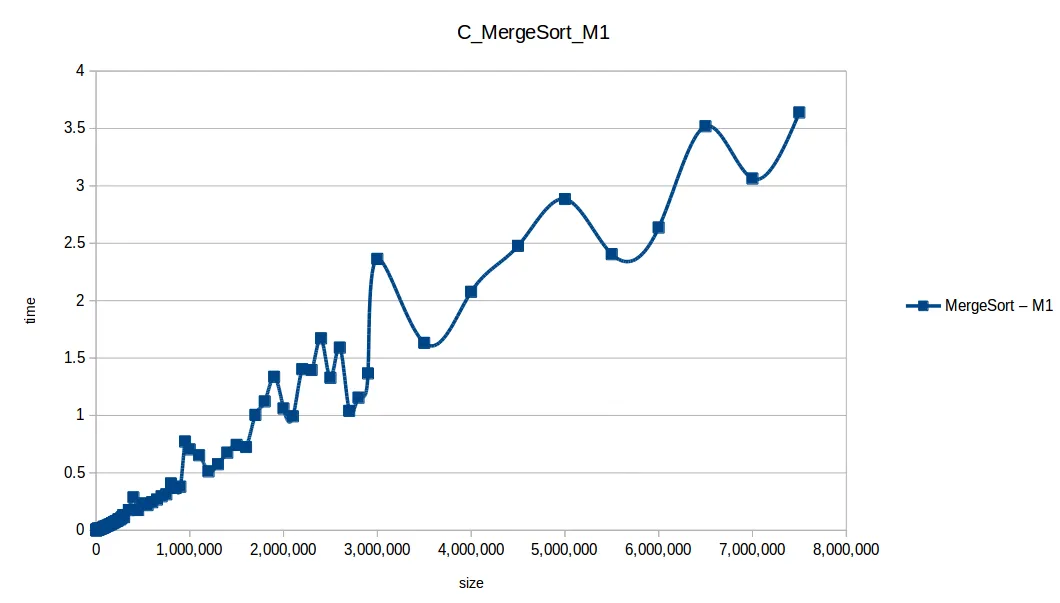
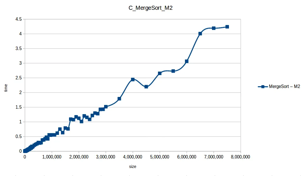
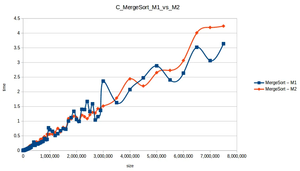
Merge Sort at max scale
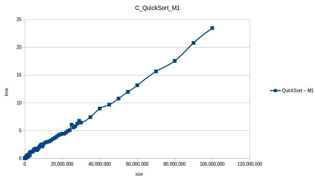
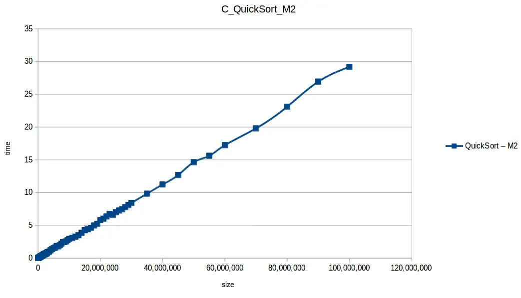
Quick Sort at max scale
Final fast-algorithm comparison
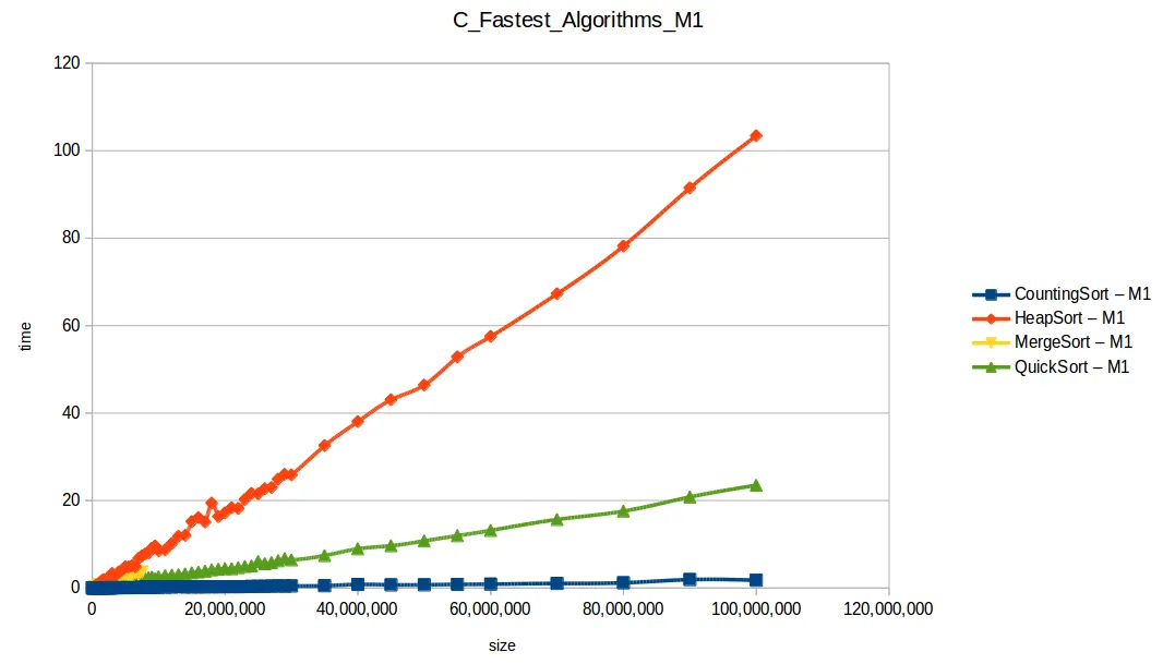
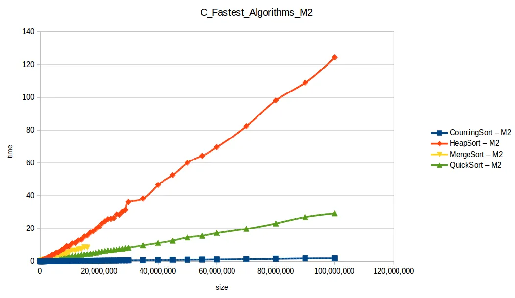
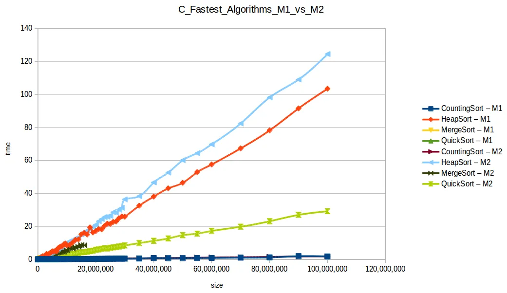
With larger input volumes, curves became more stable and easier to compare against theoretical complexity behavior.
Closing thoughts
This exercise reinforced a few core lessons:
- Algorithmic complexity matters, but implementation and hardware context matter too.
- Extra RAM may not speed single-threaded runs directly, but it can increase practical dataset limits.
- More cores do not help unless the implementation is actually parallel.
If you are getting started in computer science, I hope this serves as a useful reference.
Resources: GitHub repository
“Intelligence consists not only in knowledge, but also in the skill to apply knowledge in practice.”
Aristotle

Sergio Alexander Florez Galeano
CTO & Co-founder at DailyBot
Colombian software engineer and entrepreneur (DailyBot, YC S21). I write about AI agents, developer tools, startups, and the craft of software engineering — and I build this site in the open at XergioAleX.com.
Stay in the loop
Get notified when I publish something new. No spam, unsubscribe anytime.
No spam. Unsubscribe anytime.